16  Plots solutions

16.1 Line graph solution

Below is the code and the plot:

#Produce the plot with vectors created inside the function
plot(x = rep(1:10, 2), 
     y = seq(from = 0.5, to = 10, by = 0.5),
     col = "red",
     main = 'A line graph with "red" as the colour',
     type = "l")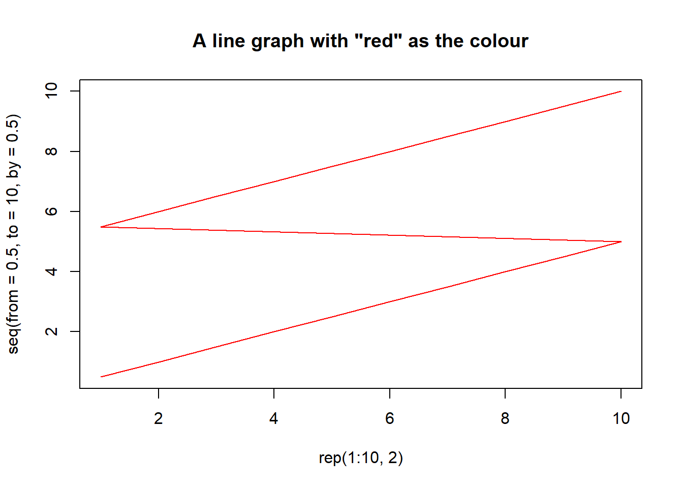

16.2 Histogram solution

Below is the code and the plot:

#Create data frame with only the Penguins from Torgersen
penguins_torgensen_df <- penguin_df[penguin_df$island == "Torgersen",]
#Create a column with body mass in kilograms
penguins_torgensen_df$body_mass_kg <- 
  penguins_torgensen_df$body_mass_g / 1000
#Plot the histogram
hist(penguins_torgensen_df$body_mass_kg,
     main = "Histogram of the body mass of Penguins from Torgersen Island",
     xlab = "Body mass in kilograms",
     ylab = "frequency",
     col = "blue")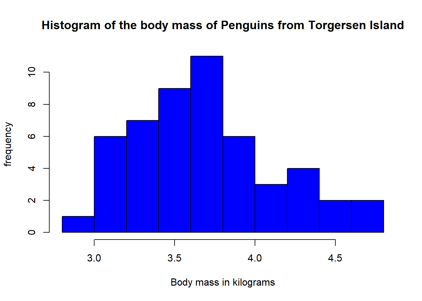

16.3 Scatterplot solution

Below is the code and the plot:

#Create data frame with only the Penguins from 2009
penguin_2009_df <- penguin_df[penguin_df$year == "2009",]
#Produce plot
plot(x = penguin_2009_df$bill_length_mm,
     y = penguin_2009_df$bill_depth_mm,
     col = as.numeric(penguin_2009_df$species),
     main = "Penguin bills vs depth in 2009",
     xlab = "Bill length (mm)",
     ylab = "Bill depth (mm)",
     pch = 15)
#Create legend
legend(x = "bottomleft", 
       col = 1:nlevels(penguin_2009_df$species),
       legend = levels(penguin_2009_df$species),
       pch = 15)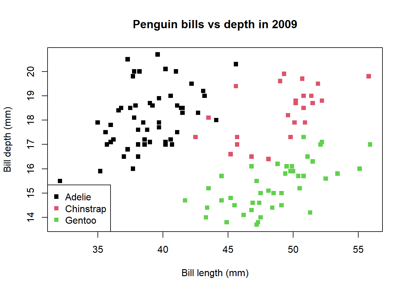

To save the plot the code is:

#Create data frame with only the Penguins from 2009
penguin_2009_df <- penguin_df[penguin_df$year == "2009",]
#Start png function
png(filename = "Chapter_13-16/Penguins_2009_bill_depth_vs_length_scatterplot.png",
    units = "mm", height = 250, width = 250, res = 150 )
#Produce plot
plot(x = penguin_2009_df$bill_length_mm,
     y = penguin_2009_df$bill_depth_mm,
     col = as.numeric(penguin_2009_df$species),
     main = "Penguin bills vs depth in 2009",
     xlab = "Bill length (mm)",
     ylab = "Bill depth (mm)",
     pch = 15)
#Create legend
legend(x = "bottomleft", 
       col = 1:nlevels(penguin_2009_df$species),
       legend = levels(penguin_2009_df$species),
       pch = 15)
#Save file
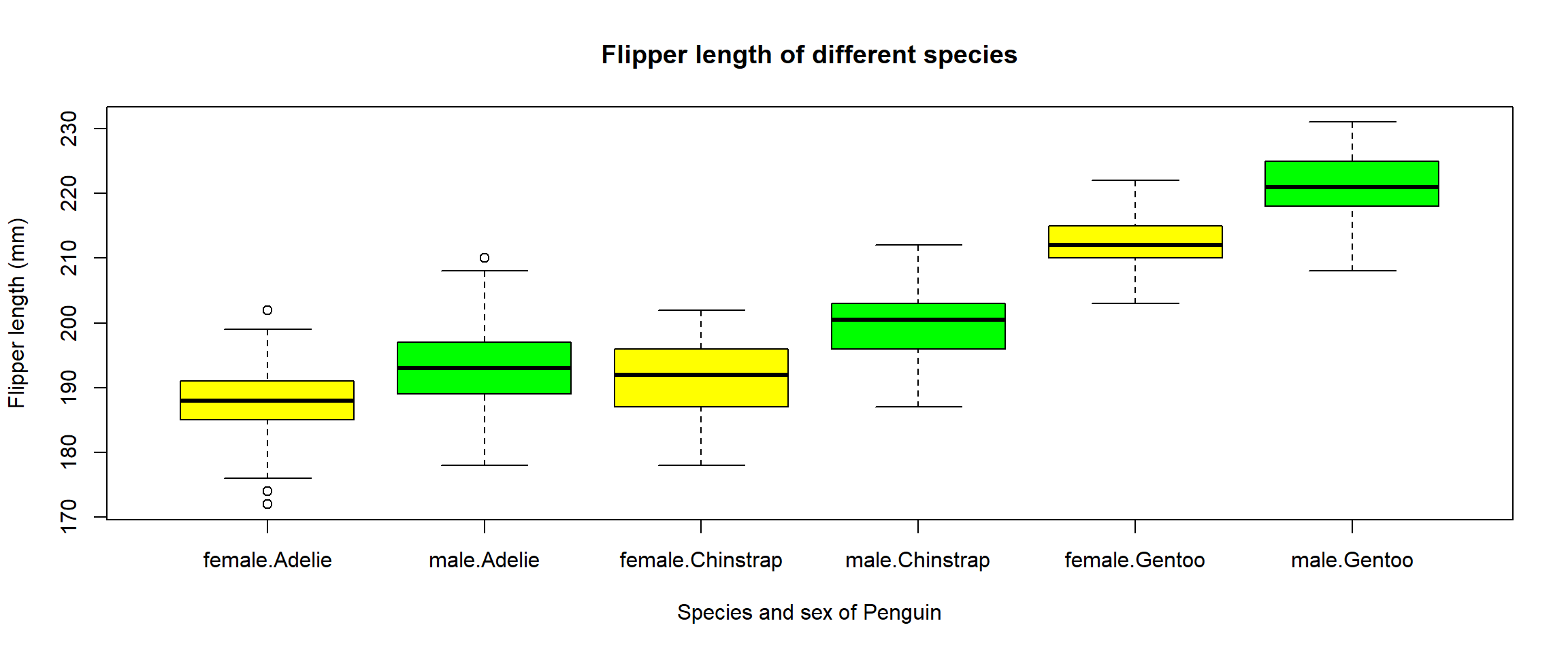
dev.off()

16.4 Boxplot solutions

Below is the code and the plot:

#Produce boxplot
boxplot(flipper_length_mm~sex*species,
        data = penguin_df,
        col = c("yellow","green"),
        main = "Flipper length of different species",
        xlab = "Species and sex of Penguin",
        ylab = "Flipper length (mm)"
)

To save the plot the code is:

#Start png function
jpeg(filename = "Chapter_13-16/Penguins_species_and_flipper_length_boxplot.jpg",
    units = "mm", height = 250, width = 300, res = 150 )
#Produce boxplot
boxplot(flipper_length_mm~sex*species,
        data = penguin_df,
        col = c("yellow","green"),
        main = "Flipper length of different species",
        xlab = "Species and sex of Penguin",
        ylab = "Flipper length (mm)"
)
#Save file
dev.off()