
19 Stats solutions
19.1 World happiness report solutions
- Read in the file
happy_df <- read.csv("Chapter_17-18/world_happiness_report_2016.csv",
                      check.names = FALSE,
                      stringsAsFactors = TRUE,
                      sep = ","
)- Answer the following questions using the output from one function:
summary(happy_df) Country Region Happiness Rank
Afghanistan: 1 Sub-Saharan Africa :38 Min. : 1.00
Albania : 1 Central and Eastern Europe :29 1st Qu.: 40.00
Algeria : 1 Latin America and Caribbean :24 Median : 79.00
Angola : 1 Western Europe :21 Mean : 78.98
Argentina : 1 Middle East and Northern Africa:19 3rd Qu.:118.00
Armenia : 1 Southeastern Asia : 9 Max. :157.00
(Other) :151 (Other) :17
Happiness Score Lower Confidence Interval Upper Confidence Interval
Min. :2.905 Min. :2.732 Min. :3.078
1st Qu.:4.404 1st Qu.:4.327 1st Qu.:4.465
Median :5.314 Median :5.237 Median :5.419
Mean :5.382 Mean :5.282 Mean :5.482
3rd Qu.:6.269 3rd Qu.:6.154 3rd Qu.:6.434
Max. :7.526 Max. :7.460 Max. :7.669
Economy (GDP per Capita) Family Health (Life Expectancy)
Min. :0.0000 Min. :0.0000 Min. :0.0000
1st Qu.:0.6702 1st Qu.:0.6418 1st Qu.:0.3829
Median :1.0278 Median :0.8414 Median :0.5966
Mean :0.9539 Mean :0.7936 Mean :0.5576
3rd Qu.:1.2796 3rd Qu.:1.0215 3rd Qu.:0.7299
Max. :1.8243 Max. :1.1833 Max. :0.9528
Freedom Trust (Government Corruption) Generosity
Min. :0.0000 Min. :0.00000 Min. :0.0000
1st Qu.:0.2575 1st Qu.:0.06126 1st Qu.:0.1546
Median :0.3975 Median :0.10547 Median :0.2225
Mean :0.3710 Mean :0.13762 Mean :0.2426
3rd Qu.:0.4845 3rd Qu.:0.17554 3rd Qu.:0.3119
Max. :0.6085 Max. :0.50521 Max. :0.8197
Dystopia Residual
Min. :0.8179
1st Qu.:2.0317
Median :2.2907
Mean :2.3258
3rd Qu.:2.6646
Max. :3.8377
- How many countries are in the region “Western Europe”?
- 21
- What is the maximum number in the “Happiness Score” column?
- 7.526
- From the columns “Economy (GDP per Capital)” to “Dystopia Residual”, which has the highest mean and which has the lowest?
- Highest: “Dystopia Residual” with 2.3258
- Lowest: “Family” with 0.13762
3.Produce the plot
#Fit linear model of Economy (x) against Family (y)
fit_economy_family <-
  lm(Family~`Economy (GDP per Capita)`, data = happy_df)
#Create string for linear equation
c <- round(fit_economy_family$coefficients[1], digits = 4)
m <- round(fit_economy_family$coefficients[2], digits = 4)
lm_equation <- paste0("y = ", m , "x + ", c)
#Produce plot
plot(x = happy_df$`Economy (GDP per Capita)`,
     y = happy_df$Family,
     main = "Comparison of the effect of \n Economy and Family on happiness",
     xlab = "Economy (GDP per Capita)",
     ylab = "Family",
     pch = as.numeric(happy_df$Region),
     xlim = c(0,2), ylim = c(0,1.5),
     col = 1)
#Add abline
abline(fit_economy_family, col = "mediumslateblue")
#Add equation to top right
text(x = 0.4, y = 1.1, labels = lm_equation)
#Add the legend
legend(x = "bottomright",
       pch = 1:nlevels(happy_df$Region),
       legend = levels(happy_df$Region))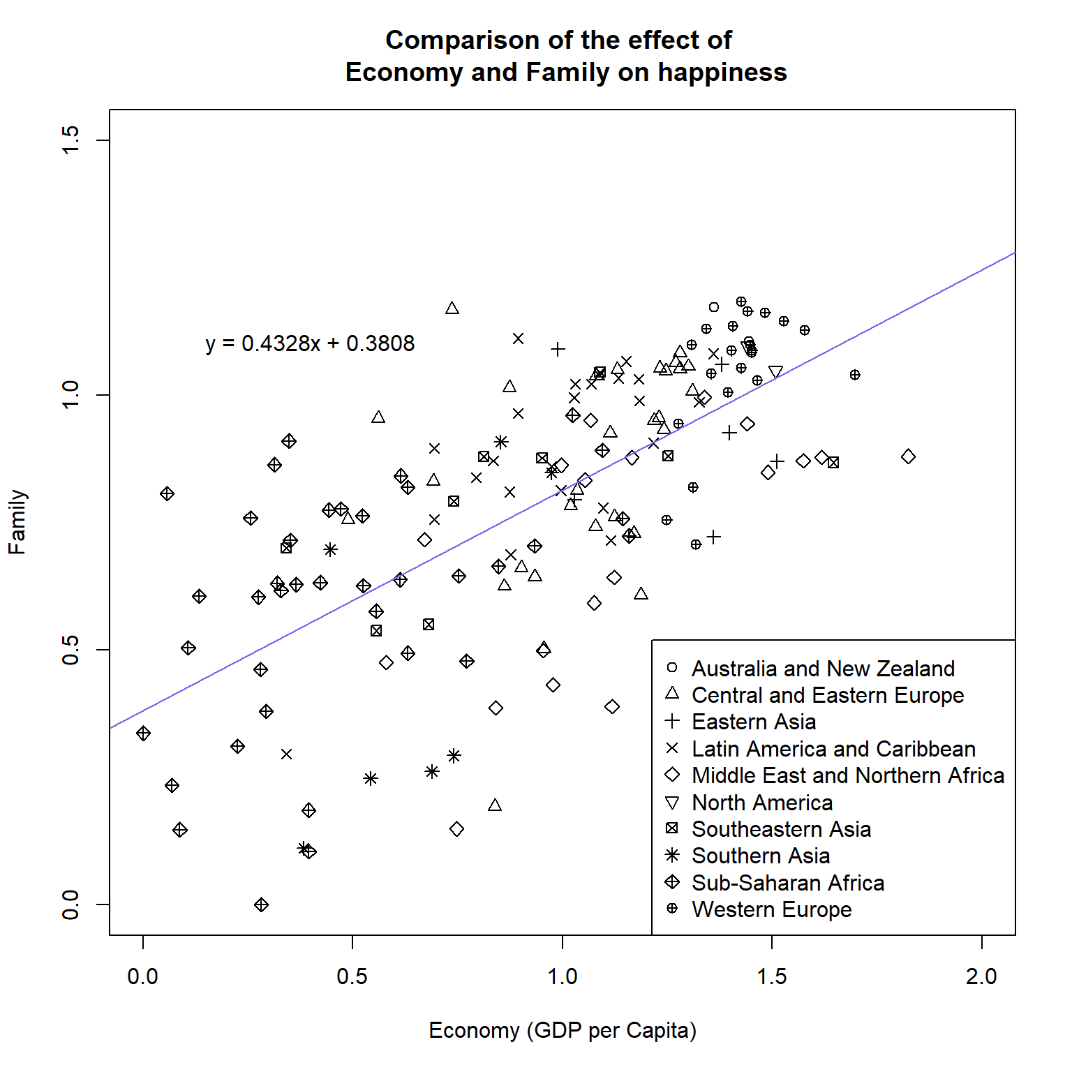
- Save plot as png file
#PNG command
png(filename = "Chapter_17-18/Economy_vs_family.png",
    units = "in", height = 8, width = 8, res = 200)
#Produce plot
plot(x = happy_df$`Economy (GDP per Capita)`,
     y = happy_df$Family,
     main = "Comparison of the effect of \n Economy and Family on happiness",
     xlab = "Economy (GDP per Capita)",
     ylab = "Family",
     pch = as.numeric(happy_df$Region),
     xlim = c(0,2), ylim = c(0,1.5),
     col = 1)
#Add abline
abline(fit_economy_family, col = "mediumslateblue")
#Add equation to top right
text(x = 0.4, y = 1.1, labels = lm_equation)
#Add the legend
legend(x = "bottomright",
       pch = 1:nlevels(happy_df$Region),
       legend = levels(happy_df$Region))
#dev.off
dev.off()- Answers for the following questions:
- Does the linear model have a positive or negative gradient?
- Positive (m = 0.4328)6
- Which variable (Economy or Family) has higher values?
- Economy
- If the value of Economy was 2.1 what would be the predictive value of Family according to the linear model equation?
- __(0.4328*2.1) + 0.3808 = 1.28968__
- Which region appears to have the highest values for Economy and for Family?
- Western Europe
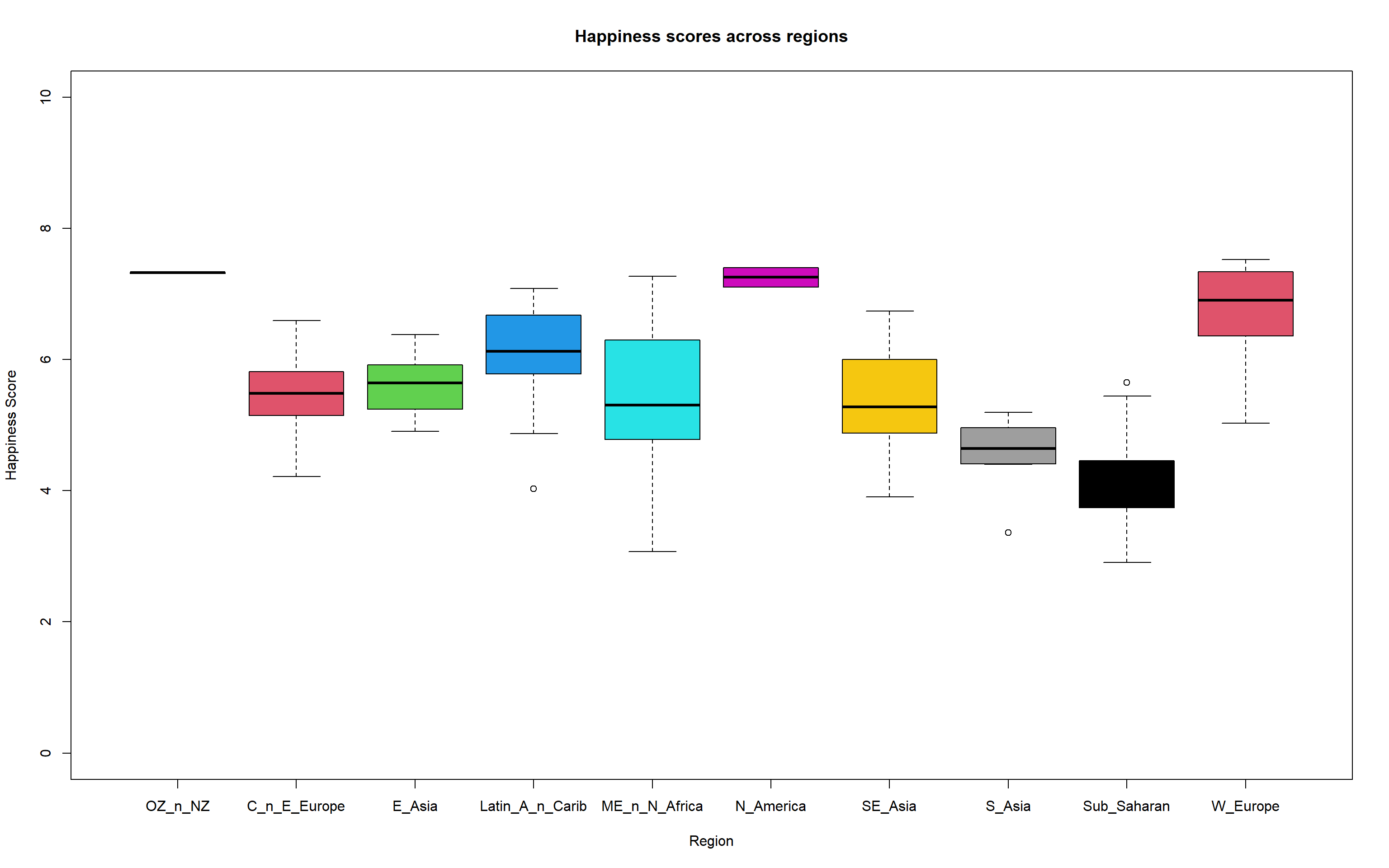
- Produce boxplot
#Change level names
short_region_names <-
  c("OZ_n_NZ", "C_n_E_Europe", "E_Asia", "Latin_A_n_Carib",
    "ME_n_N_Africa", "N_America", "SE_Asia", "S_Asia",
    "Sub_Saharan", "W_Europe")
levels(happy_df$Region) <- short_region_names
#Create boxplot
boxplot(`Happiness Score`~Region, data = happy_df,
        ylim = c(0,10),
        col = 1:nlevels(happy_df$Region),
        main = "Happiness scores across regions"
)
- Save as jpeg
#jpeg
jpeg(filename = "Chapter_17-18/Region_happiness_boxplots.jpg", units = "px",
     width = 1500, height = 750 )
#Create boxplot
boxplot(`Happiness Score`~Region, data = happy_df,
        ylim = c(0,10),
        col = 1:nlevels(happy_df$Region),
        main = "Happiness scores across regions"
)
#dev.off
dev.off()- T-tests
#Subset the data frames to get vectors of our regions of interest
WE_happiness <- happy_df[happy_df$Region == "W_Europe","Happiness Score"]
NA_happiness <- happy_df[happy_df$Region == "N_America","Happiness Score"]
SA_happiness <- happy_df[happy_df$Region == "S_Asia","Happiness Score"]
SEA_happiness <- happy_df[happy_df$Region == "SE_Asia","Happiness Score"]
#Carry out t-tests
WE_NA_ttest <- t.test(WE_happiness, NA_happiness)
WE_SA_ttest <- t.test(WE_happiness, SA_happiness)
SA_SEA_ttest <- t.test(SA_happiness, SEA_happiness)
#Extract p values into a new vector with element names
region_happiness_pvalues <- c(WE_NA = WE_NA_ttest$p.value,
                              WE_SA = WE_SA_ttest$p.value,
                              SA_SEA = SA_SEA_ttest$p.value)
#Logical to determine if the p-value is less than 0.05
#I.e. the means are significantly different
region_happiness_pvalues < 0.05
WE_NA WE_SA SA_SEA
FALSE TRUE FALSE