Chapter 3 Figure 3
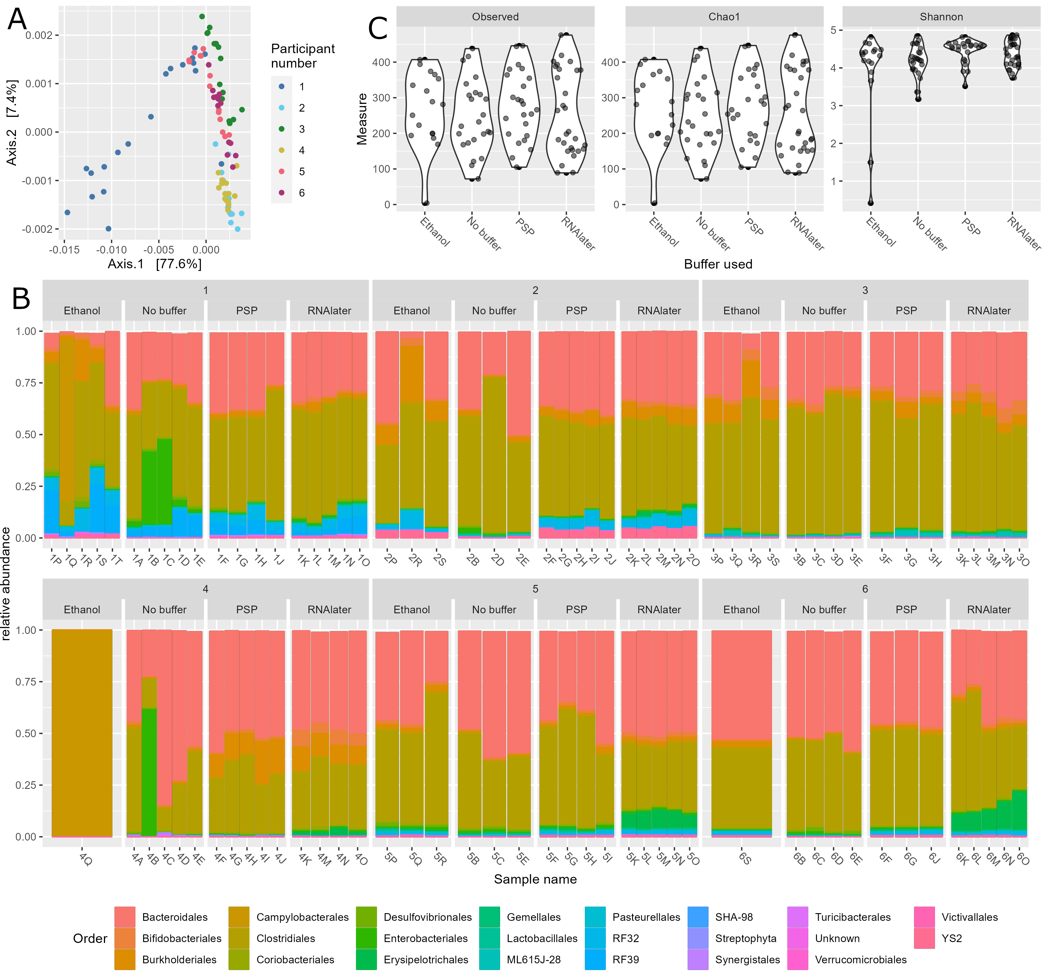
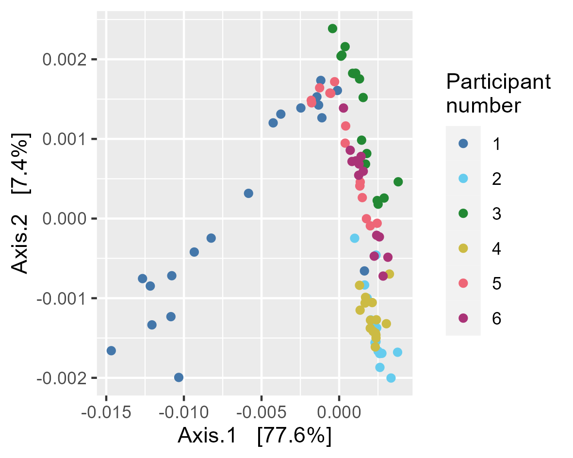
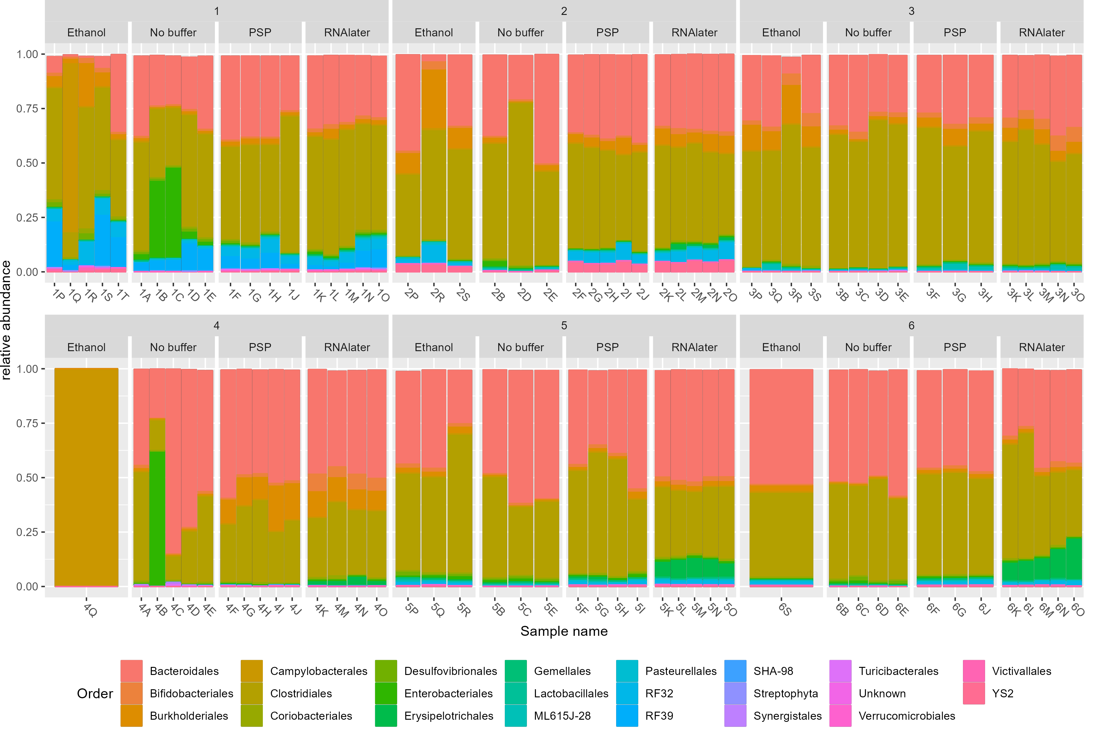
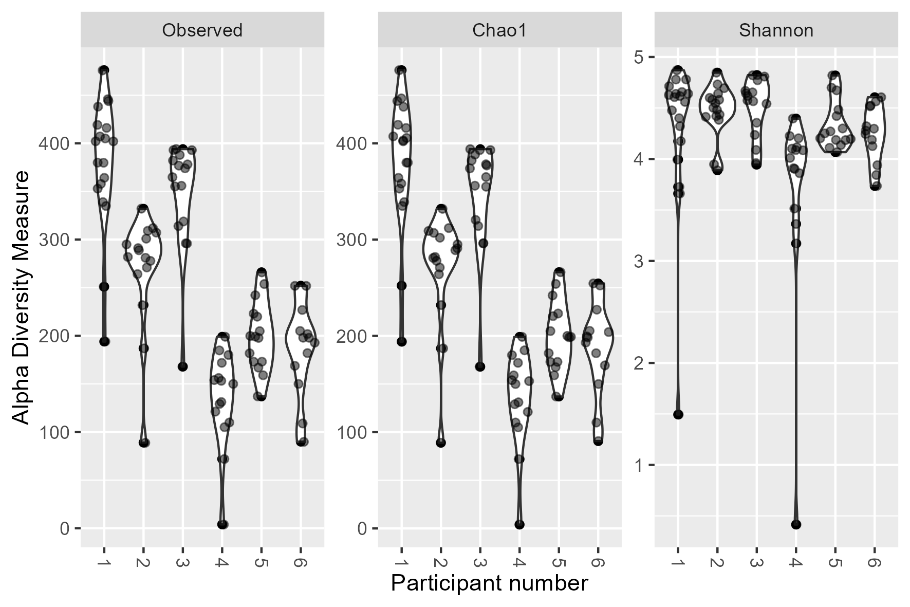
Gut microbiota composition in study subjects. (A) Principal component analysis of stool microbiota composition based on DADA2 produced ASVs. (B) Relative abundance at the order level derived from 16S rRNA gene sequences within each sample. Bar charts are faceted by participant (1–6) and buffer used metadata information. (C) Diversity (observed species, chao1 and Shannon) of the microbiota of stool samples stratified by storage buffer (ethanol, no buffer, PSP buffer, RNAlater).

3.2 Figure 3A
#Load in data
load("./data/preprocess_physeq")

#Transform samples to even sampling depth
physeq <- transform_sample_counts(physeq,
                                  function(x) 30000 * x/sum(x))
#Save object
save(physeq, file = "./data/preproces_physeq_even_depth30k")
#load in phyloseq object
load("./data/preproces_physeq_even_depth30k")

#Produce Weighted unifrac oridnation
ord <- ordinate(physeq, "PCoA", "wunifrac")

#Use Paul Tol colour blind palette
tol_pal <- c("#4477AA","#66CCEE","#228833","#CCBB44","#EE6677","#AA3377")

#Create plot
p <-  plot_ordination(physeq, ord,
                      color="Patientnumber") +
  scale_color_manual(values=tol_pal)+
  #Change legend title to Participant number
  labs(colour="Participant\nnumber")

#Save plot
ggsave(plot = p,
       "./figures/weighted_unifrac_patient.png",
       device = "png", units = "mm", height = 80, width = 100,
       dpi = 300)
3.3 Figure 3B
#Load in relative abundance phyloseq
load("./data/physeq_relabund")

#Aggregate taxa to order
physeq_order_relabund <- aggregate_taxa(physeq_relabund, 'Order')
#Remove Appearing square brackets again
tax_table(physeq_order_relabund)[,] <- gsub(pattern = "\\[" , replacement = "", tax_table(physeq_order_relabund)[,])
tax_table(physeq_order_relabund)[,] <- gsub(pattern = "\\]" , replacement = "", tax_table(physeq_order_relabund)[,])
row.names(tax_table(physeq_order_relabund)) <- gsub(pattern = "\\[" , replacement = "", row.names(tax_table(physeq_order_relabund)))
row.names(tax_table(physeq_order_relabund)) <- gsub(pattern = "\\]" , replacement = "", row.names(tax_table(physeq_order_relabund)))

order_taxa_df <- as.data.frame(tax_table(physeq_order_relabund))

#Produce plot
p <- plot_bar(physeq_order_relabund, x = "Sample_name", fill = "Order")+
  geom_bar(aes(color=Order, fill=Order), stat="identity", position="stack") +
  facet_nested_wrap(~Patientnumber+Bufferused, nrow = 2, scales = "free_x") +
  theme(legend.position="bottom",
        axis.text.x = element_text(
          angle = -45, vjust = 0.5, hjust=0.1),
        plot.margin = margin(0,5,0,0, "mm"),
        panel.spacing.x=unit(0.2, "lines")) +
  labs(x= "Sample name", y = "relative abundance") +
  guides(fill=guide_legend(ncol=8))

#Save plot
ggsave(plot = p,filename = "./figures/order_relabund_facet_buffer.png",
       device = "png", units = "mm", height = 200, width = 300,
       dpi=300)
3.3.1 Percentage of Bacteroides and Firmicutes
#Load in relative abundance phyloseq
load("./data/physeq_relabund")

#Aggregate taxa to order
physeq_phylum_relabund <- aggregate_taxa(physeq_relabund, 'Phylum')

#Extract abundance table
df <- abundances(physeq_phylum_relabund)

#Create vector of relabund of bact and Firm added
Bac_firm_vec <- df["Bacteroidetes",] + df["Firmicutes",]

samples <- names(Bac_firm_vec[Bac_firm_vec < 0.5])

metadf <- as.data.frame(meta(physeq_phylum_relabund))

meta_samples <- metadf[metadf$Sample_name %in% samples,]
3.4 Figure 3C
#load in phyloseq object
load("./data/preprocess_physeq")

#Produce plot
p <- plot_richness(physeq, x = "Bufferused",
                   measures = c("Observed","Chao1","Shannon")) +
  geom_violin() +
  ggforce::geom_sina(alpha=0.5) +
  theme(legend.position="none",
        axis.text.x = element_text(
          angle = -45, vjust = 0.5, hjust=0.1)) +
  labs(x= "Buffer used", y = "Measure")

#Save plot
ggsave(plot = p,
       filename = "./figures/alpha_diversity_patient.png",
       device = "png", units = "mm", height = 80, width = 200)