Chapter 5 Figure 5

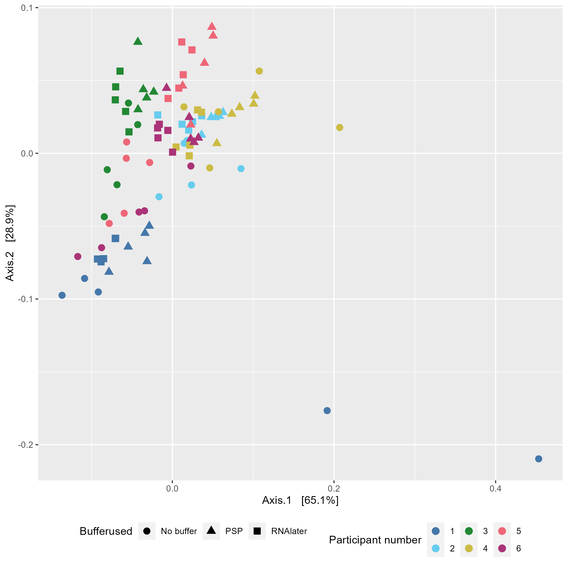
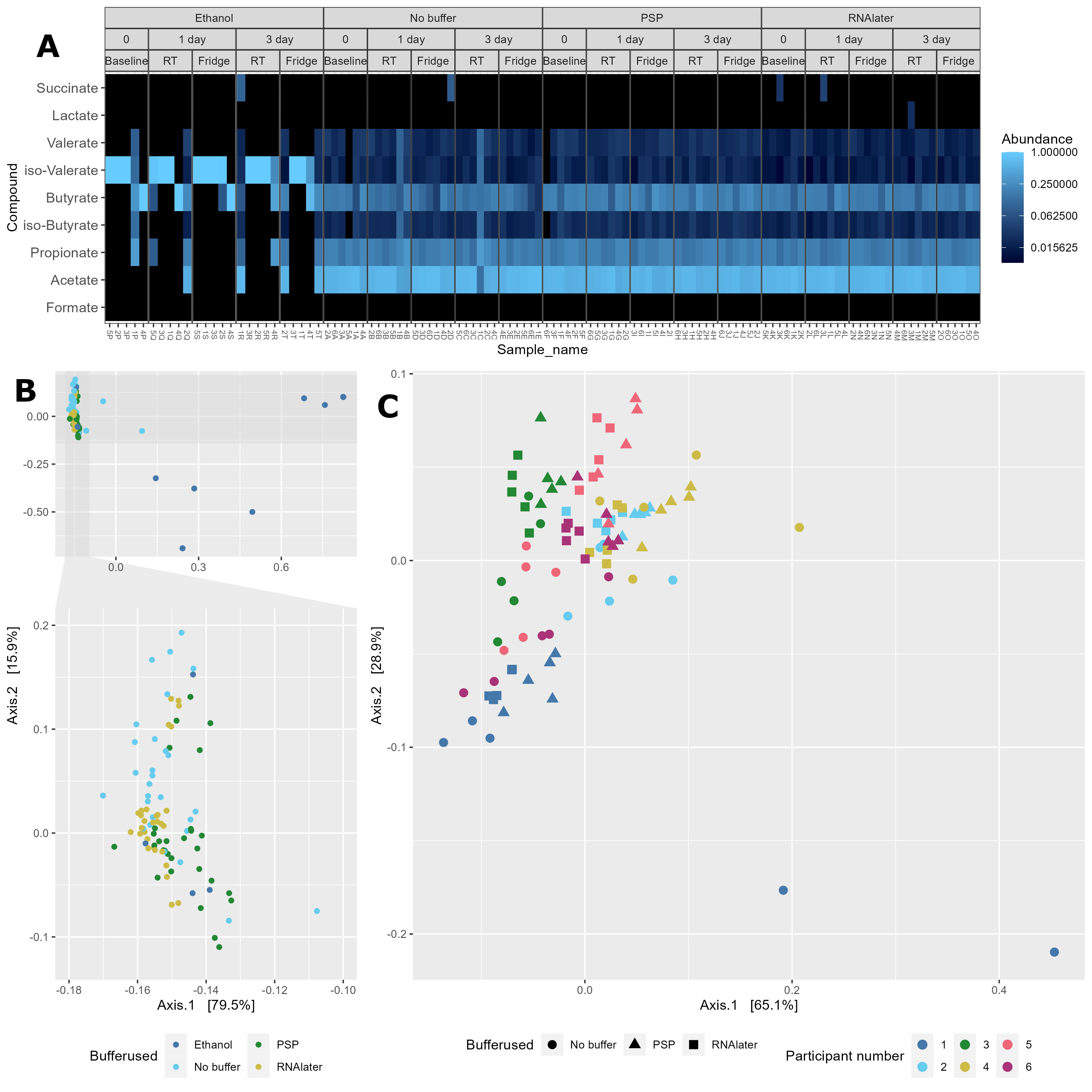
GC-MS derived SCFA profiles in study samples. (A) Relative abundance of SCFAs in study samples faceted based on the type of buffer used (Ethanol, No buffer, PSP buffer, or RNAlater). (B) Bray-Curtis based principal component analysis (PCoA) of stool SCFA composition (set to even sampling depth of 1000) stratified by participant and storage temperature (Baseline:–80oC, Fridge:4oC or RT:20oC). Bottom plots are zoomed in sections to display clustering without outliers. (C) Bray-Curtis based PCoA excluding ethanol samples of stool SCFA composition (set to even sampling depth of 1000) stratified by storage time and temperature (Baseline:–80oC, Fridge:4oC or RT:20oC).

5.1 libraries

library("ggplot2")
library("phyloseq")
library("tidyverse")
library("dplyr")
library("vegan")
library("reshape2")
library("ggplot2")
library("ggh4x")
library("patchwork")
library("ggforce")
library("ggpubr")

5.2 Preprocess data

#Load phyloseq
load(file = "data/lipid_physeq_object")

#Set to even sampling depth
#Set to even sampling depth (1000)
physeq_1k = transform_sample_counts(physeq, 
                                    function(x) 1000 * x/sum(x))

#save physeq object
save(physeq_1k, file = "./data/lipid_physeq_1k_object")

5.3 Colour blindy friendly palettes

tol_pal <- c("#4477AA","#66CCEE","#228833","#CCBB44","#EE6677","#AA3377")

5.4 A Heatmap

#Choose order for temp
#sample_data(physeq_1k)[,"Temp"] <- factor(sample_data(physeq_1k)[,"Temp"], levels = c("Baseline", "RT", "Fridge"))


#Make relative abundance physeq
physeq_relabund <- microbiome::transform(physeq, "compositional")

#Heatmap
heatmap_facet <- 
  plot_heatmap(physeq_relabund,
               sample.label = "Sample_name", 
               taxa.label = "Compound") +
  facet_nested( ~ Buffer.type + Storage.time + Temp , scales = "free_x") +
  theme(panel.spacing.x=unit(0, "lines")) +
   theme(axis.text.x = element_text(size=6))
  
ggsave(plot = heatmap_facet, 
       filename = "figures/lipid_heatmap.png", 
       device = "png", dpi = 300,
       units = "mm", width = 300, height = 100)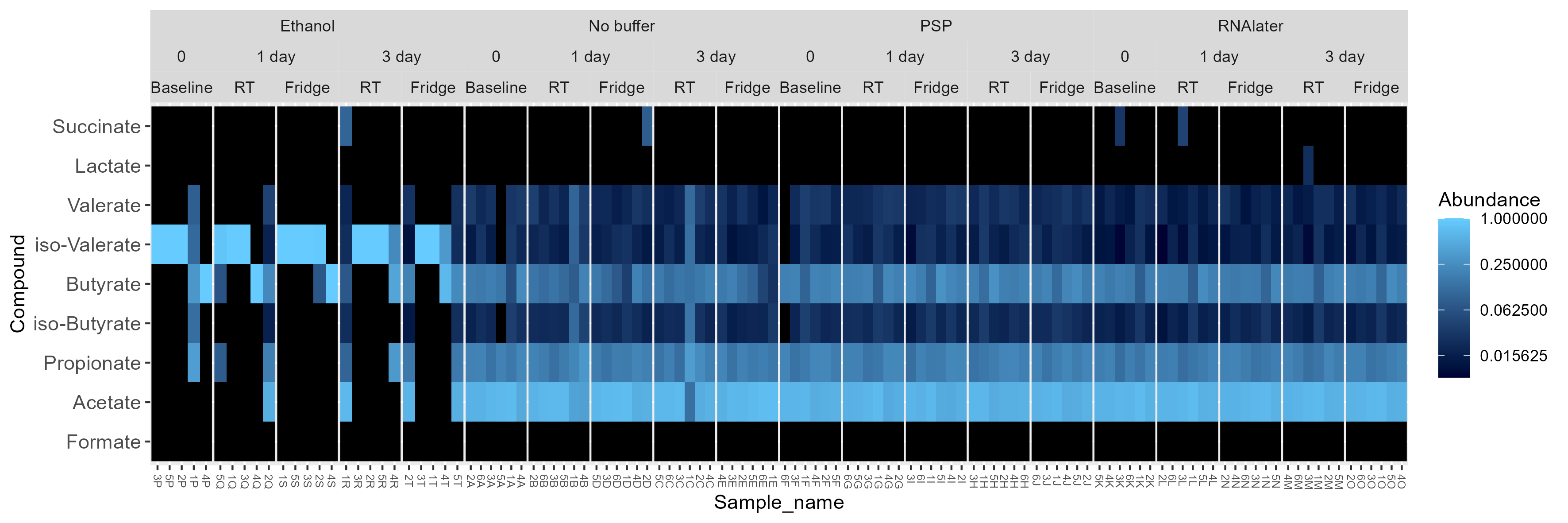

5.5 B & C

#PCoA bray curtis ordination
physeq_1k_ord_pcoa_bray <- ordinate(physeq_1k, "PCoA", "bray")

5.5.1 B PCoA plot

All sample PCoA to show clustering by buffer

#NMDS_bray facetted by Buffer.type.Temp, shape by sample
NMDS_bray_facet <- 
  plot_ordination(physeq_1k, physeq_1k_ord_pcoa_bray,
                  color = "Buffer.type") +
  scale_color_manual(values=tol_pal) +
  labs(colour="Bufferused") +
  theme(legend.position="bottom") +
  guides(color = guide_legend(nrow=2)) +
  facet_zoom(xlim = c(-0.18,-0.10), ylim=c(-0.125,0.2), horizontal = FALSE)
ggsave(NMDS_bray_facet,
       filename = "./figures/Lipids_PCoA_bray_curtis_colour_by_buffer.png",
       device = "png", dpi = 300,
       units = "mm", width = 100, height = 200)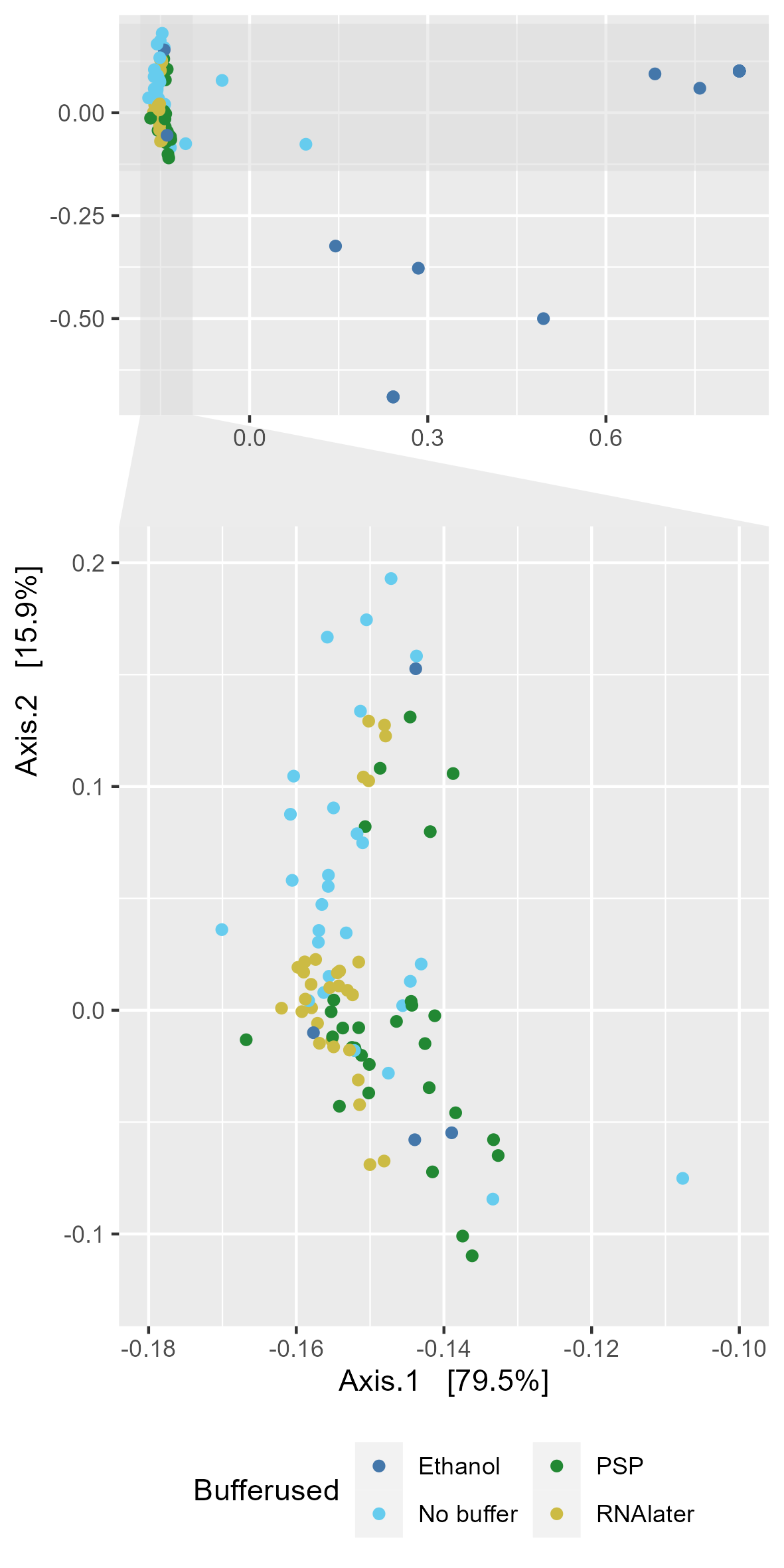

5.5.2 C PCoA plot

Plot without ethanol

5.6 Without ethanol

#subset physeq to remove ethanol
physeq_1k_no_ethanol <- phyloseq::subset_samples(physeq_1k, Buffer.type %in% c("No buffer","PSP","RNAlater"))
#NMDs bray curtis
physeq_1k_ord_pcoa_bray_no_ethanol <- ordinate(physeq_1k_no_ethanol, "PCoA", "bray")

No ethanol colour by participant and shape by buffer

#NMDS_bray facetted by Buffer.type.Temp, shape by sample
NMDS_bray_facet <- 
  plot_ordination(physeq_1k_no_ethanol, physeq_1k_ord_pcoa_bray_no_ethanol,
                  color = "Sample.number", shape = "Buffer.type") +
  geom_point(size=3) +
  scale_color_manual(values=tol_pal) +
  labs(colour="Participant number", shape="Bufferused") +
  theme(legend.position="bottom")
ggsave(NMDS_bray_facet,
       filename = "./figures/Lipids_PCoA_bray_curtis_colour_by_participant_shape_by_buffer_no_ethanol.png",
       device = "png", dpi = 300,
       units = "mm", width = 200, height = 200)