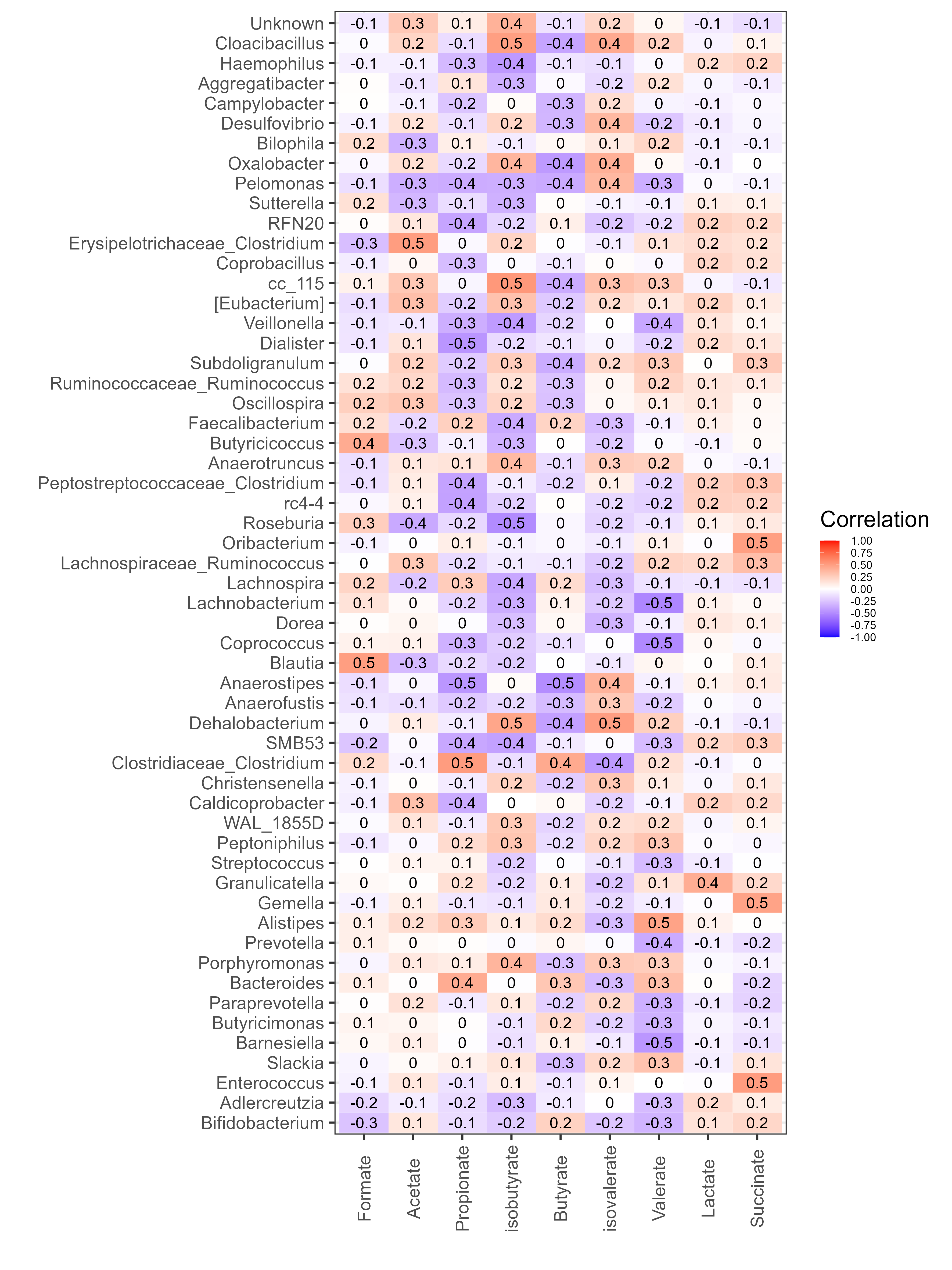
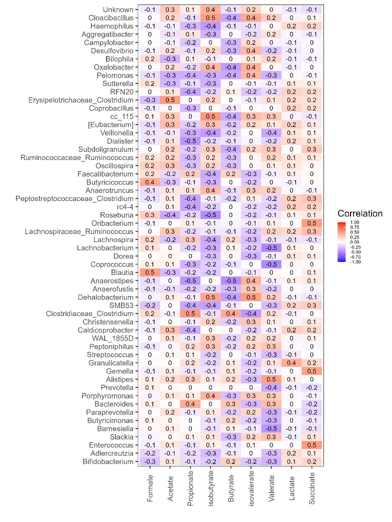
Chapter 6 Figure 6
Correlation of bacterial genera with SCFA metabolites. Spearman’s correlation was carried out on all the samples with matching ASV (≥4,528 reads) and SCFA data. Relative abundance values of SCFAs and genera were used for correlation. Only genera with significant correlations are displayed (adjusted p-value (fdr) <0.05), all correlation values between the SCFAs and these genera are displayed. The y-axis represents the SCFA metabolites. The x-axis represents the genera of bacteria (based on 16S rRNA gene sequences). Red and blue indicate positive and negative correlation, respectively.
Created with assistance of tutorial: https://microbiome.github.io/tutorials/Heatmap.html
6.2 Preprocess tables
#load in phyloseq object
load("./data/preprocess_physeq")
#subset samples to remove rnalater unwashed samples
physeq <-
  subset_samples(physeq, !(RNAlater_washed_status == "unwashed"))
#Subset samples to remove samples with NA lipid info
physeq <- subset_samples(physeq, !(Formate.MM. == "NA"))
#Remove anything that is not bacteria
physeq <- subset_taxa(physeq, Phylum != "Bacteria")

#Clostridium
#Get logical vector to know which rows
clos_subset_vector <- as.vector(replace((tax_table(physeq)[,"Genus"] == "Clostridium"),
        is.na(tax_table(physeq)[,"Genus"] == "Clostridium"),
        FALSE))
#Extract taxa names
clos_taxa_names <- taxa_names(physeq)[clos_subset_vector]
#Make new genus names for clositriudm
clos_new_genus_name <- paste(tax_table(physeq)[clos_taxa_names,"Family"],
                             tax_table(physeq)[clos_taxa_names,"Genus"],
                             sep = "_")
tax_table(physeq)[clos_taxa_names,"Genus"] <- clos_new_genus_name
#Ruminococcus
#Remove instances of square brackets
clos_subset_vector <- as.vector(replace((tax_table(physeq)[,"Genus"] == "[Ruminococcus]"),
        is.na(tax_table(physeq)[,"Genus"] == "[Ruminococcus]"),
        FALSE))
#Remove []
clos_taxa_names <- taxa_names(physeq)[clos_subset_vector]
tax_table(physeq)[clos_taxa_names,"Genus"] <- "Ruminococcus"
#Get logical vector to know which rows
clos_subset_vector <- as.vector(replace((tax_table(physeq)[,"Genus"] == "Ruminococcus"),
        is.na(tax_table(physeq)[,"Genus"] == "Ruminococcus"),
        FALSE))
#Extract taxa names
clos_taxa_names <- taxa_names(physeq)[clos_subset_vector]
#Make new genus names for clositriudm
clos_new_genus_name <- paste(tax_table(physeq)[clos_taxa_names,"Family"],
                             tax_table(physeq)[clos_taxa_names,"Genus"],
                             sep = "_")
tax_table(physeq)[clos_taxa_names,"Genus"] <- clos_new_genus_name


#Convert to genus table
physeq <- aggregate_taxa(physeq, "Genus")
#COnvert to relative abundance
physeq_relabund <- microbiome::transform(physeq, "compositional")
#Extract genus table to a df
genus_df <- as.matrix(otu_table(physeq_relabund))
#transpose
genus_df_t <- as.matrix(t(genus_df))
#log10 the values
#genus_df_t_log10 <- log10(genus_df_t)

#extract lipid table
lipid_mat <-
  as.matrix(meta(physeq)[,grepl(".MM.",colnames(meta(physeq)))])
#remove .MM. from colnames
colnames(lipid_mat) <-
  gsub(pattern = ".MM.", replacement = "", colnames(lipid_mat))
#Remove "_b" from sample names
row.names(lipid_mat) <- gsub(pattern = "_b", replacement = "",
                             row.names(lipid_mat))
row.names(genus_df_t) <- gsub(pattern = "_b", replacement = "",
                             row.names(genus_df_t))
#Convert to relative abundance values
lipid_mat_relabund <- make_relative(lipid_mat)

#Save object
save(genus_df_t, file = "./data/16s_and_lipid_genus_physeq")
save(lipid_mat_relabund, file = "./data/lipid_relabund_matrix")
6.3 All buffers
6.3.1 Correlation
#load in phyloseq object
load("./data/16s_and_lipid_genus_physeq")
load("./data/lipid_relabund_matrix")
#Correlation
correlation.table <- associate(
  genus_df_t,
  lipid_mat_relabund,
  method = "spearman", mode = "table",
  p.adj.threshold = 0.05, n.signif = 1)
#Add column names
colnames(correlation.table)[1:2] <- c("Genus","Lipid")
#Write table with significant hits to file
write.table(correlation.table[correlation.table$p.adj < 0.05,],
            file = "./data/Genus_lipid_sig_correlation.csv",
            row.names = FALSE, sep = ",", quote = FALSE,
            col.names = TRUE)
#Create wide table of sig correlations
long_df <- correlation.table[correlation.table$p.adj < 0.05,]
#Remove p.adj value
long_df <- long_df[,-4]
#long to wide
wide_df <- dcast(long_df, Genus ~ Lipid, value.var = "Correlation")
#Write to file
write.table(wide_df,
file = "./data/Genus_lipid_sig_correlation_wide.csv",
row.names = FALSE, sep = ",", quote = FALSE,
col.names = TRUE)6.3.2 Heatmap
theme_set(theme_bw(20))
df <- correlation.table
p <- ggplot(df, aes(Genus, Lipid, group=Lipid))
p <- p + geom_tile(aes(fill = Correlation))
p <- p + geom_text(aes(label = round(df$Correlation, 1)), size = 5)
p <- p +
  scale_fill_gradientn("Correlation",
                       breaks = seq(from = -1, to = 1,  by = 0.25),
                       colours = c("blue", "white", "red"),
                       limits = c(-1, 1)) +
  theme(axis.text.x = element_text(angle = 90, vjust = 0.5),
        legend.text=element_text(size=10)) +
  labs(x = "", y = "") +
  coord_flip()
ggsave(plot = p,
       filename = "./figures/Genus_lipid_corr_heatmap.png",
       device = "png", units = "mm",
       height = 400, width = 300, dpi = 300)