Chapter 4 Figure 4
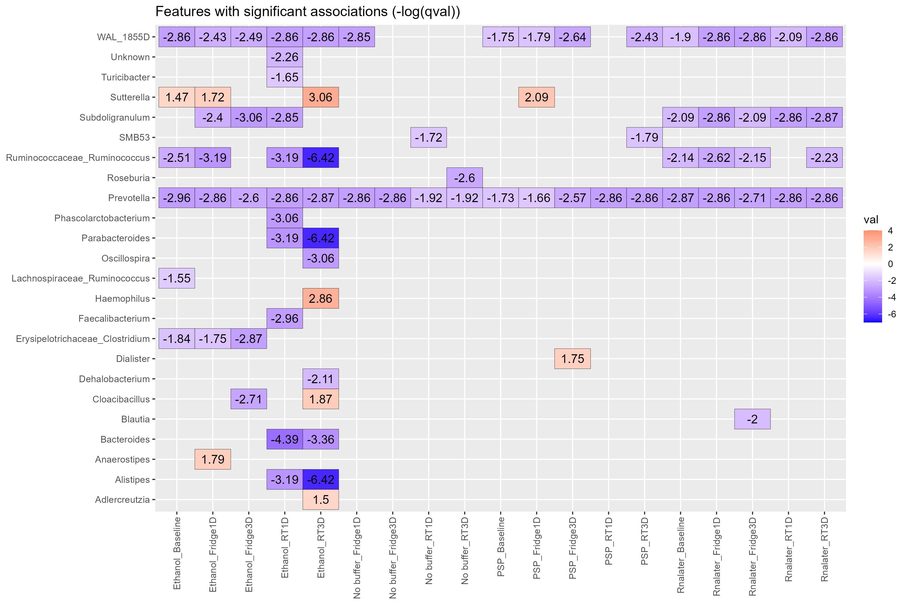
Biomarkers heatmap. Heatmap showing the genera (y-axis) with significant associations discovered by Maaslin2. Comparisons were carried out using the type of buffer used and the storage conditions metadata information (x-axis). Storage condition included Temperature (Fridge:4oC or RT:20oC) and Days stored before being frozen at -80oC (1D: One day, 3D: Three days), Baseline samples were immediately frozen at -80oC. The no buffer at Baseline:–80oC group was used as the reference. Participant numbers were used for random effects for the model. Values on heatmap are (-log(qval)*sign(coeff)).
4.2 Genus
4.2.1 Preprocess table and convert to genus table
#load in phyloseq object
load("./data/preprocess_physeq")

sample_data(physeq)

#subset samples to remove rnalater unwashed samples
physeq <- subset_samples(physeq, !(RNAlater_washed_status == "unwashed"))
#Remove anything that is not bacteria
physeq <- subset_taxa(physeq, Phylum != "Bacteria")

#Clostridium
#Get logical vector to know which rows
clos_subset_vector <- as.vector(replace((tax_table(physeq)[,"Genus"] == "Clostridium"),
        is.na(tax_table(physeq)[,"Genus"] == "Clostridium"),
        FALSE))
#Extract taxa names
clos_taxa_names <- taxa_names(physeq)[clos_subset_vector]
#Make new genus names for clositriudm
clos_new_genus_name <- paste(tax_table(physeq)[clos_taxa_names,"Family"],
                             tax_table(physeq)[clos_taxa_names,"Genus"],
                             sep = "_")
tax_table(physeq)[clos_taxa_names,"Genus"] <- clos_new_genus_name
#Ruminococcus
#Remove instances of square brackets
clos_subset_vector <- as.vector(replace((tax_table(physeq)[,"Genus"] == "[Ruminococcus]"),
        is.na(tax_table(physeq)[,"Genus"] == "[Ruminococcus]"),
        FALSE))
#Remove []
clos_taxa_names <- taxa_names(physeq)[clos_subset_vector]
tax_table(physeq)[clos_taxa_names,"Genus"] <- "Ruminococcus"
#Get logical vector to know which rows
clos_subset_vector <- as.vector(replace((tax_table(physeq)[,"Genus"] == "Ruminococcus"),
        is.na(tax_table(physeq)[,"Genus"] == "Ruminococcus"),
        FALSE))
#Extract taxa names
clos_taxa_names <- taxa_names(physeq)[clos_subset_vector]
#Make new genus names for clositriudm
clos_new_genus_name <- paste(tax_table(physeq)[clos_taxa_names,"Family"],
                             tax_table(physeq)[clos_taxa_names,"Genus"],
                             sep = "_")
tax_table(physeq)[clos_taxa_names,"Genus"] <- clos_new_genus_name


#Create
#Convert to genus table
physeq <- aggregate_taxa(physeq, "Genus")
#transform to relabund
physeq_relabund <- abundances(physeq, "compositional")
# Get data into maaslin format ####
#First need df of relabund
df_data <- t(as.data.frame(otu_table(physeq_relabund, taxa_are_rows=TRUE)))
#next metadata
#the nonsense is so it becomes a normal df
#rather than a weird phyloseq object within a df
df_metadata <-
  as.data.frame(t(t(as.data.frame(sample_data(physeq)))))
#keep only columns of interest
df_metadata <- df_metadata[,c(2,5,10,11,12,13)]
#convert some columns to numeric
df_metadata$Storagetemp <- as.numeric(df_metadata$Storagetemp)
df_metadata$DaysstoredpriortoDNAextraction <- as.numeric(df_metadata$DaysstoredpriortoDNAextraction)
df_metadata$DNAconcng_ul <- as.numeric(df_metadata$DNAconcng_ul)
#remvo phyloseq object
rm(physeq)
rm(physeq_relabund)
#Edit metadata
df_metadata$Bufferused_and_Storageconditions <-
  paste0(df_metadata$Bufferused, "_", df_metadata$Storageconditions)
#Remove unwanted metadata columns
df_metadata <- df_metadata[,c(1,5,7)]
#Convert all columns to factors columns
df_metadata[] <- lapply( df_metadata, factor)

#Save objects
save(df_data, file = "./data/maaslin_genus_df")
save(df_metadata, file = "./data/maaslin_genus_metadata")
4.2.2 MaAsLin2 on genera
#Remove Days stored info
df_metadata <- df_metadata[,c(1,3)]
#fit data
fit_data <- Maaslin2::Maaslin2(input_data = df_data,
                     input_metadata = df_metadata,
                     output = "standard_maaslin2_genus",
                     #Random sample used for subject/patients
                     random_effects = "Patientnumber",
                     reference = c("Bufferused_and_Storageconditions", "No buffer_-80")
                     )
#Create heatmap of significant results
#Read in data
df <- read.csv(
file = "./standard_maaslin2_genus/significant_results.tsv",
sep = "\t", check.names=FALSE)
#Create (-log(qval)*sign(coeff)) column for value
df$val <- (-log(df$qval)*sign(df$coef))
#Create min and max val
lo <- floor(min(df$val))
up <- ceiling(max(df$val))
mid <- 0
#Change -80 to Baseline
df$value <- gsub(pattern = "_-80", replacement = "_Baseline", df$value)
#Create rounded value for text
df$val_round <- round(df$val, digits = 2)
#heatmap
heatmap_media <- ggplot(df,
aes(x = value, y = feature, fill = val)) +
#Produce ggplot as tile/heatmap style plot
ggplot2::geom_tile(colour = "black") +
#Customise colour gradient
ggplot2::scale_fill_gradient2(low = "blue", high = "red", mid = "white",
na.value = "white",
midpoint = mid, limit = c(lo,up)) +
#Add the values as text in the cells
ggplot2::geom_text(aes(value, feature, label = val_round),
colour = "black", size = 4) +
#Remove the x and y labels (NULL) and add a title
ggplot2::labs(x = NULL, y = NULL,
title = "Features with significant associations (-log(qval))") +
theme(axis.text.x = element_text(angle = 90, vjust = 0.5, hjust=1))
ggsave(filename = "./figures/maaslin2_heatmap_genus.png", plot = heatmap_media,
device = "png", dpi = 300, units = "mm", height = 200, width = 300)